Using Deep Learning to detect Pneumonia in X-ray images
Using Pytorch to develop a Deep Learning framework to predict pneumonia in X-ray images
- About
- Import libraries
- Colab setup and getting data from Kaggle
- Data exploration
- Visualisation
- Transfer Learning model (Resnet34 model with our custom classifier)
- Setup the Training (and Validation) model
- Run the Training (and Validation) model
- Testing
-
Lessons Learned
About
This blog is towards the Course Project for the [Pytorch Zero to GANS] free online course(https://jovian.ml/forum/c/pytorch-zero-to-gans/18) run by JOVIAN.ML.
The course competition was based on analysing protein cells with muti-label classification.
Therefore, to extend my understanding of dealing with medical imaging I decided to use the X-Ray image database in Kaggle.
Seeing as I ran out of GPU hours on Kaggle because of the competition (restricted to 30hrs/week at the time of writing June 2020) I opted to use Google Colab.
This blog is in the form of a Jupyter notebook and inspired by link.
The blog talks about getting the dataset in Google Colab, explore the dataset, develop the training model, metrics and then does some preliminary training to get a model which is then used to make a few predictions. I will then talk about some of the lessons learned.
Warning! The purpose of this blog is to outline the steps taken in a typical Machine Learning project and should be treated as such.
The full notebook on Google Colab is here. It is worth taking a peek just to see the monokai UI as snippet of which is whon below:
Import libraries
import os
import torch
import pandas as pd
import time
import copy
import PIL
import numpy as np
from torch.utils.data import Dataset, random_split, DataLoader
from PIL import Image
import torchvision
from torchvision import datasets
import torchvision.models as models
import matplotlib.pyplot as plt
from tqdm.notebook import tqdm
import torchvision.transforms as T
from sklearn.metrics import f1_score
import torch.nn.functional as F
import torch.nn as nn
from torch.optim import lr_scheduler
from collections import OrderedDict
from torchvision.utils import make_grid
from torch.autograd import Variable
import seaborn as sns
import csv
%matplotlib inline```
Colab setup and getting data from Kaggle
I used Google Colab with GPU processing for this project because I had exhausted my Kaggle hours (30hrs/wk) working on the competition :( The challenge here was signing into Colab, setting up the working directoty and then linking to Kaggle and copying the data over. The size of the dataset was about 1.3Gb which wasn’t too much of a bother as Google gives each Gmail account 15Gb for free!
Tip: I used the monokai settings in Colab which gave excellent font contrast and colours for editing.

from google.colab import drive
drive.mount('/content/drive', force_remount=True)
The default directory that is linked to the Google’s gdrive ( the one connected to the gmail address) is /content/drive/My Drive/
I create a project directory jovian-xray and use this as the new root directory.
root_dir = '/content/drive/My Drive/jovian-xray'
os.chdir(root_dir)
!pwd
os.mkdir('kaggle')
Install Kaggle in your current Colab session. Log into Kaggle, point to the dataset and copy the API key. This downloads a kaggle.json file. Upload this kaggle.json to Colab.
!pip install -q kaggle from google.colab import files
Select the kaggle.json file. This will be uploaded to your current working directory which is the root_dir as specified above. Create a ./kaggle directory in the home directory Copy the kaggle.json from the current directory to this new directory. Change permissions so that it can be executed by user and group.
upload = files.upload() !mkdir ~/.kaggle !ls !cp kaggle.json ~/.kaggle/ !chmod 600 ~/.kaggle/kaggle.json
proj_dir = os.path.join(root_dir, 'kaggle', 'chest_xray')
os.chdir(proj_dir)
!pwd
In the Kaggle data directory page select New Notebook > Three vertical dots, Copy API Command
#API key !kaggle datasets download -d paultimothymooney/chest-xray-pneumonia
!unzip chest-xray-pneumonia
os.listdir(proj_dir)
The dataset is structured into training, val and test folders, each with sub-folders of NORMAL and PNEUMONIA images.
Data exploration
Image transforms
We will now prepare the data for reading into Pytorch as numpy arrays using DataLoaders.
Havig data augmentation is a good way to get extra training data for free. However, care must be taken to ensure that the transforms requested are likely to appear in the inference (or test set).
The images (RGB) are normalized using the mean [0.485,0.456,0.406] and standard deviation [0.229,0.224,0.225] of that used for the Imagenet data in the Resnet model, so that the new input images have the same distribution and mean as that used in the Resnet model.
I have set up two transforms dictionaries, one with and one without so it would be easy to plot images and compare.
imagenet_stats = ([0.485, 0.456, 0.406], [0.229, 0.224, 0.225])

data_transforms = {'train' : T.Compose([
    T.Resize(224),
    T.CenterCrop(224),
    T.RandomRotation(20),
    T.RandomHorizontalFlip(),
    T.ToTensor(),
    T.Normalize(*imagenet_stats, inplace=True)
]),
'test' : T.Compose([
    T.Resize(224),
    T.CenterCrop(224),
    T.ToTensor(),
    T.Normalize(*imagenet_stats, inplace=True)
]),
'val' : T.Compose([
    T.Resize(224),
    T.CenterCrop(224),
    T.ToTensor(),
    T.Normalize(*imagenet_stats, inplace=True)
])}

data_no_transforms = {'train' : T.Compose([ T.ToTensor() ]),
'test' : T.Compose([T.ToTensor() ]),
'val' : T.Compose([T.ToTensor() ])}
Dataloaders
image_datasets = {x: datasets.ImageFolder(os.path.join(proj_dir, x),
                                          data_transforms[x]) for x in ['train', 'val','test']}

# Using the image datasets and the transforms, define the dataloaders
dataloaders = {x: torch.utils.data.DataLoader(image_datasets[x], batch_size=4,
                                             shuffle=True, num_workers=2) for x in ['train', 'val','test']}

dataset_sizes = {x: len(image_datasets[x]) for x in ['train', 'val']}


class_names= image_datasets['train'].classes

print(class_names)
op: [‘NORMAL’, ‘PNEUMONIA’]
Processed Images print(image_datasets[‘train’][0][0].shape) print(image_datasets[‘train’])
op:
op: torch.Size([3, 224, 224])
Dataset ImageFolder
Number of datapoints: 5216
Root location: /content/drive/My Drive/jovian-xray/kaggle/chest_xray/train
StandardTransform
Transform: Compose(
Resize(size=224, interpolation=PIL.Image.BILINEAR)
CenterCrop(size=(224, 224))
RandomRotation(degrees=(-20, 20), resample=False, expand=False)
RandomHorizontalFlip(p=0.5)
ToTensor()
Normalize(mean=[0.485, 0.456, 0.406], std=[0.229, 0.224, 0.225])
)
Visualisation
The image data is converted in to Numpy arrays and then treated with the mean and std so that we can view the images as seen by the model.
def imshow(img, title=None):
    img = img.numpy().transpose((1, 2, 0))
    img = np.clip(img, 0, 1)
    plt.imshow(img)
    if title is not None:
        plt.title(title)

def raw_imshow(img, title=None):
    img = img.numpy().transpose((1, 2, 0))
    mean = np.array([0.485, 0.456, 0.406])
    std = np.array([0.229, 0.224, 0.225])
    img = std * img + mean
    img = np.clip(img, 0, 1)
    plt.imshow(img)
    if title is not None:
        plt.title(title)

# Get a batch of training data
images, classes = next(iter(dataloaders['train']))
# Make a grid from batch
out = torchvision.utils.make_grid(images)
plt.figure(figsize=(8, 8))
raw_imshow(out, title=[class_names[x] for x in classes])

Transfer Learning model (Resnet34 model with our custom classifier)
The method of transfer learning is widely used to take advantage of the clever and hardworking chaps who have spent time to train a model on million+ images and save the trained model architecture and weights.
The Resnet34 model has been trained on the Imagenet database which has 1000 classes from trombones to toilet tissue.
Resnet34 has a top-most fully connected layer to predict 1000 classes. In our case we need only two so we will remove the last fc layer and add our own.
Have a look here for a good explanation of Resnet architectures. Briefly, the after each set of convolutions the input is added to the output. This helps to maintain the reslotion of the input, ie do not lose any features of the input model.
In a deep neural network the early layers capture generic features such as edges, texture and colour while the latter layers capture more specific features such as cats ears, eyes, elephant trunks and so on.
So our process is take the trained resnet architecture and weights, remove the head ie the last layers that are used to predict the 1000 classes and add our own tailored to the number of classes we want to predict, which in our case is two.
We will do a first pass of training where the weights of the resnet model are locked ie, ie we do not want to overwrite or lose those values which will mean more GPU expense for us. Then we will unfreeze the weights and run the entire model at our prefereed laerning rate. Note, idelaly we would like to unfreeze only specific layer, say layer 1 and layer 4, which I will cover in a separate blogpost.
Build and train your network
Load resnet-34 pre-trained network
model = models.resnet34(pretrained=True)
op: The tailed output of the model summary gives:
) (avgpool): AdaptiveAvgPool2d(output_size=(1, 1)) (fc): Linear(in_features=512, out_features=1000, bias=True) ) In the Resnet34 architecture the final fully connected layer has in_features and 1000 out_features for the 1000 classes. But we need only two output classes.
So we add two linear layers to go from 512 RELU 256 and then 256 LOGSOFTMAX to 2 classes
Use a LogSoftmax for the final classification activation.
from collections import OrderedDict classifier = nn.Sequential(OrderedDict([ (‘fc1’, nn.Linear(2048, 1024)), (‘relu’, nn.ReLU()), (‘fc2’, nn.Linear(1024, 2)), (‘output’, nn.LogSoftmax(dim=1)) ]))
Replacing the pretrained model classifier with our classifier
model.fc = classifier
def freeze(model):
  # To freeze the residual layers
  for param in model.parameters():
    param.requires_grad = False
  for param in model.fc.parameters():
    param.requires_grad = True

def unfreeze(self):
  # Unfreeze all layers
  for param in model.parameters():
    param.requires_grad = True
freeze(model)
Count the trainable parameters to make sure we only include our new head. cp = count_parameters(model) print(f’{cp} trainable parameters in frozen model ‘)
op: 131842 trainable parameters in frozen model
Check: (512 * 256 + 256 bias) + (256 * 2 + 2 bias)
Setup the Training (and Validation) model
The dataset has training, val and tests which makes our lives a little bot easier ie we don’t have to do any data splitting and can set up specific transforms for each.
Training the model
def train_model(model, criterion, optimizer, scheduler, num_epochs=10):
    since = time.time()

    best_model_wts = copy.deepcopy(model.state_dict())
    best_acc = 0.0

    for epoch in range(1, num_epochs+1):
        print('Epoch {}/{}'.format(epoch, num_epochs))
        print('-' * 10)

        # Each epoch has a training and validation phase
        for phase in ['train', 'val']:
            if phase == 'train':
                scheduler.step()
                model.train()  # Set model to training mode
            else:
                model.eval()   # Set model to evaluate mode

            running_loss = 0.0
            running_corrects = 0

            # Iterate over data.
            for inputs, labels in dataloaders[phase]:
                inputs, labels = inputs.to(device), labels.to(device)

                # zero the parameter gradients
                optimizer.zero_grad()

                # forward
                # track history if only in train
                with torch.set_grad_enabled(phase == 'train'):
                    outputs = model(inputs)
                    loss = criterion(outputs, labels)
                    _, preds = torch.max(outputs, 1)

                    # backward + optimize only if in training phase
                    if phase == 'train':
                        loss.backward()
                        optimizer.step()

                # statistics
                running_loss += loss.item() * inputs.size(0)
                running_corrects += torch.sum(preds == labels.data)

            epoch_loss = running_loss / dataset_sizes[phase]
            epoch_acc = running_corrects.double() / dataset_sizes[phase]

            print('{} Loss: {:.4f} Acc: {:.4f}'.format(
                phase, epoch_loss, epoch_acc))

            # deep copy the model
            if phase == 'val' and epoch_acc > best_acc:
                best_acc = epoch_acc
                best_model_wts = copy.deepcopy(model.state_dict())

        print()

    time_elapsed = time.time() - since
    print('Training complete in {:.0f}m {:.0f}s'.format(
        time_elapsed // 60, time_elapsed % 60))
    print('Best valid accuracy: {:4f}'.format(best_acc))

    # load best model weights
    model.load_state_dict(best_model_wts)
    return model
Check if a GPU is available
Any Deep Learning (neural network) model must be run on a GPU because the algoritms are tailored to exploit the parallel processing capabilities of these. So a quick check is made to see if a GPU exists so that data can be sent to this. Google COlab has a seeting under Edit > Notebook Settings : Select None/GPU/TPU TPU is for Tensor Processing Unit which is even faster than GPU.
nThreads = 4
batch_size = 32
use_gpu = torch.cuda.is_available()
train_on_gpu = torch.cuda.is_available()

if not train_on_gpu:
    print('CUDA is not available.  Training on CPU ...')
else:
    print('CUDA is available!  Training on GPU ...')

device = torch.device("cuda:0" if torch.cuda.is_available() else "cpu")
print(device)
Run the Training (and Validation) model
Use the Adam optimizer which is the preferred optimizer because it is adaptive and adds a momentum element to the gradient stepping.
Train a model with a pre-trained network
num_epochs = 10
if use_gpu:
    print ("Using GPU: "+ str(use_gpu))
    model = model.cuda()
Use NLLLoss because our output is LogSoftmax criterion = nn.NLLLoss()
Adam optimizer with a learning rate
optimizer = torch.optim.Adam(model.fc.parameters(), lr=0.0001) Decay LR by a factor of 0.1 every 5 epochs exp_lr_scheduler = lr_scheduler.StepLR(optimizer, step_size=10, gamma=0.1)
Train the frozen model where the bottom layers only are frozen
model_fit = train_model(model, criterion, optimizer(lr=0.001), exp_lr_scheduler, num_epochs=10)
Unfreeze the model and train some more
unfreeze(model)
Testing
Do validation on the test set
def test(model, dataloaders, device):
  model.eval()
  accuracy = 0

  model.to(device)

  for images, labels in dataloaders['test']:
    images = Variable(images)
    labels = Variable(labels)
    images, labels = images.to(device), labels.to(device)

    output = model.forward(images)
    ps = torch.exp(output)
    equality = (labels.data == ps.max(1)[1])
    accuracy += equality.type_as(torch.FloatTensor()).mean()

    print("Testing Accuracy: {:.3f}".format(accuracy/len(dataloaders['test'])))
test(model, dataloaders, device)
Save the checkpoint
model.class_to_idx = dataloaders['train'].dataset.class_to_idx
model.epochs = num_epochs
checkpoint = {'input_size': [2, 224, 224],
                 'batch_size': dataloaders['train'].batch_size,
                  'output_size':2,
                  'state_dict': model.state_dict(),
                  'data_transforms': data_transforms,
                  'optimizer_dict':optimizer.state_dict(),
                  'class_to_idx': model.class_to_idx,
                  'epoch': model.epochs}
save_fname= os.path.join(proj_dir, '90_checkpoint.pth')
torch.save(checkpoint,  save_fname)
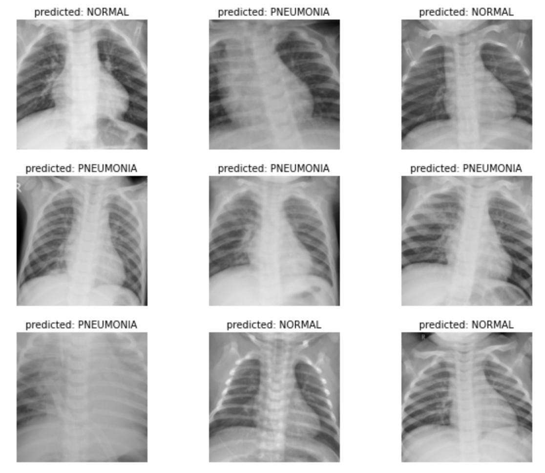
#Visualise the Training/Validation images
def visualize_model(model, num_images=6):
    was_training = model.training
    model.eval()
    images_so_far = 0
    fig = plt.figure()

    with torch.no_grad():
        for i, (inputs, labels) in enumerate(dataloaders['test']):
            inputs = inputs.to(device)
            labels = labels.to(device)

            outputs = model(inputs)
            _, preds = torch.max(outputs, 1)

            for j in range(inputs.size()[0]):
                images_so_far += 1
                ax = plt.subplot(num_images//2, 2, images_so_far)
                ax.axis('off')
                ax.set_title('predicted: {}'.format(class_names[preds[j]]))
                imshow(inputs.cpu().data[j])

                if images_so_far == num_images:
                    model.train(mode=was_training)
                    return
        model.train(mode=was_training)
visualize_model(model_ft)
print (predict('chest_xray/test/NORMAL/NORMAL2-IM-0348-0001.jpeg', loaded_model))
(array([0.96704894, 0.03295105], dtype=float32), [‘NORMAL’, ‘PNEUMONIA’])
The NORMAL probablility is much larger than the one for pneumonia.
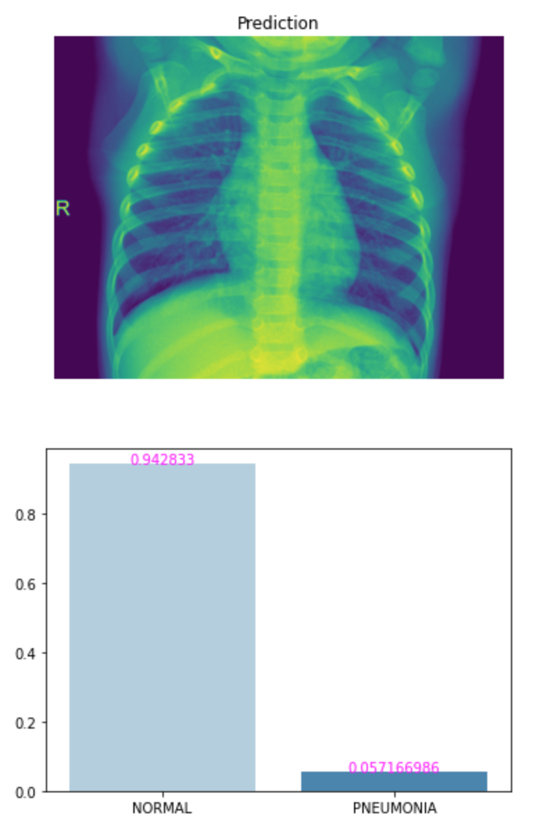
img = os.path.join(proj_dir, 'test/NORMAL/NORMAL2-IM-0337-0001.jpeg')
p, c = predict(img, loaded_model)
view_classify(img, p, c, class_names)
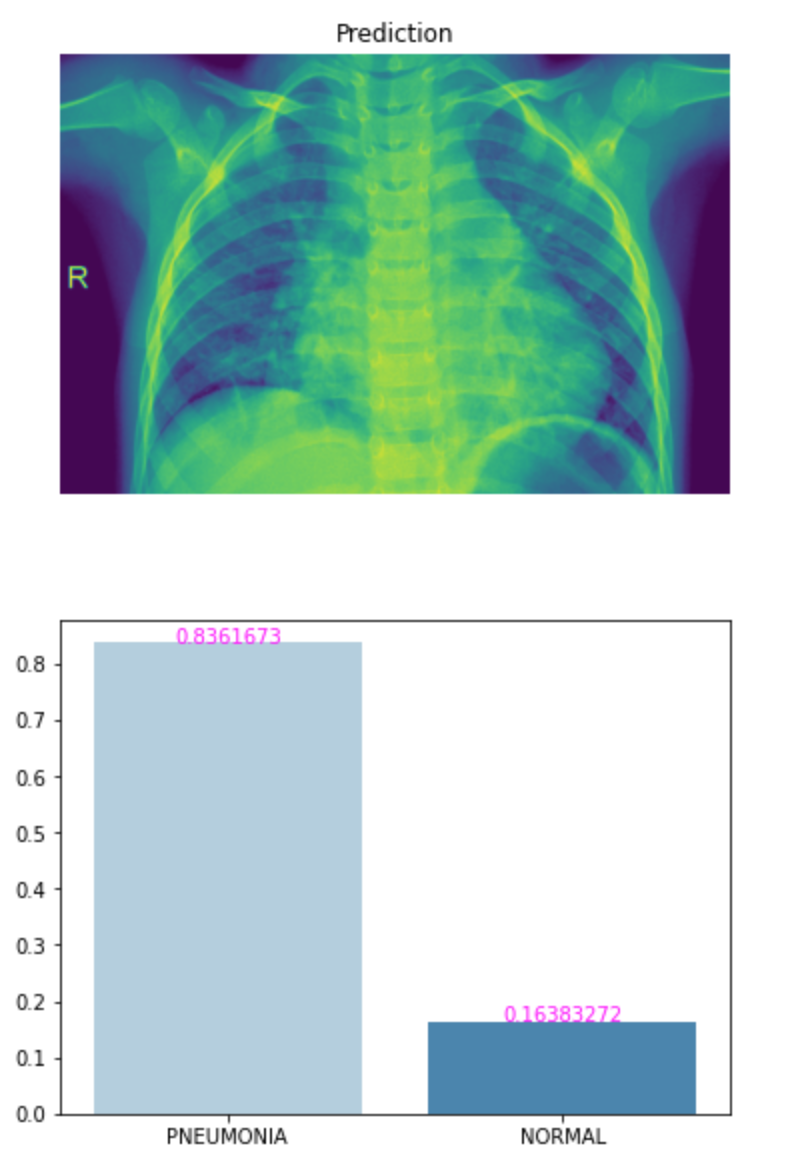
img = os.path.join(proj_dir, 'test/PNEUMONIA/person99_bacteria_474.jpeg')
p, c = predict(img, loaded_model)
view_classify(img, p, c, class_names)
Lessons Learned
- There are five methods to reduce model overfitting. Overfitting results when the model fits very well to the training data (low error) but not very well to the validation data (high error).
These are:
Get more data
Data augmentation
Generalizable architectures
Regularisation
Reduce architecture complexity -
Undertaking an online course like the Jovian Zero to Gans has been an excellent opportunity to immerse myself in Machine Learning. Taking part in the competition (which is ongoing) and writing this blog on the X-ray dataset has helped me to better understand important concepts such as Dataloaders, learning rate, batch size, optimizers and loss functions.
- Thank you to Aakash the course instructor and the rest pf the Jovian team for the efforts in helping us to better understand such an exciting paradigm.
![]()